Gráfico en R sobre la influencia de las distribuciones a priori

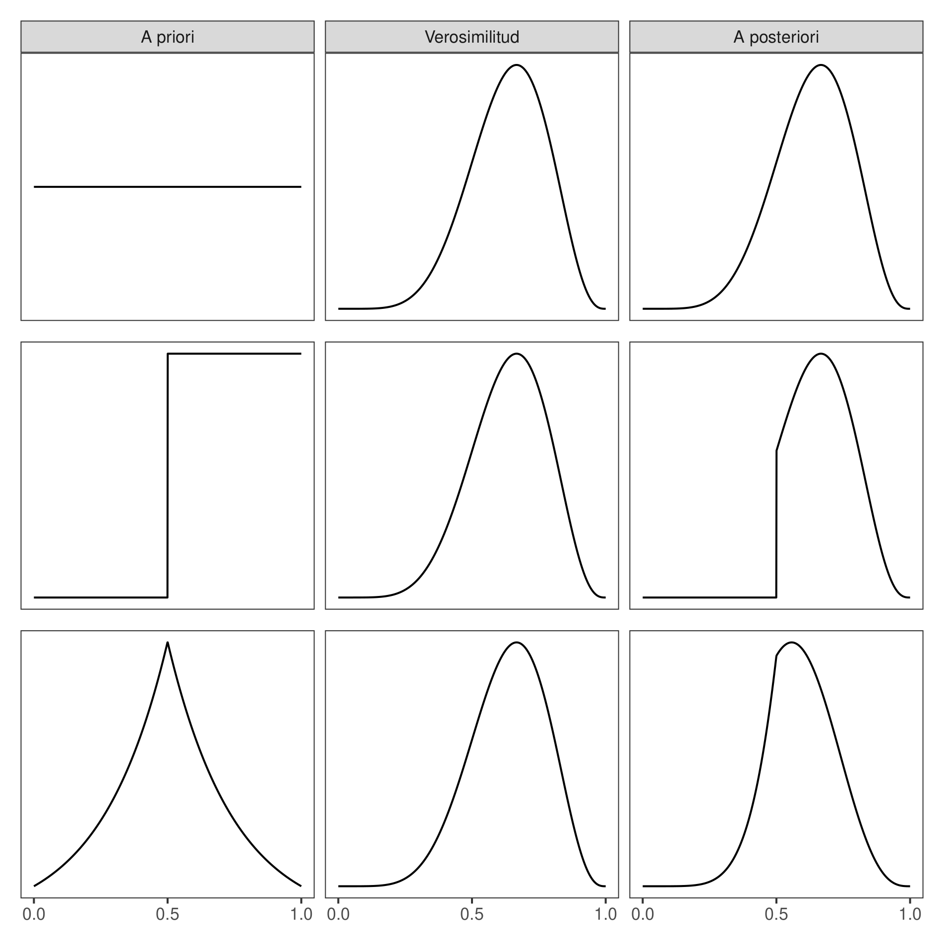
Kurz A. Solomon ha replicado en R el gráfico de McElreath, R. (2020). Statistical rethinking: A Bayesian course with examples in R and Stan (Second Edition) de CRC Press que muestra los efectos de las distribuciones a priori en el capítulo Making the Model Go, página 38.

Se comparan tres distribuciones a priori, una uniforme, una de tipo escalón y la de Laplace, donde ponderan (filtran) la función de verosimilitud (señal de entrada) dando una distribución a posteriori diferente (señal de salida).

library(tidyr)
library(ggplot2)
library(dplyr)
## Gráfico de Statistical Rethinking, Making the Model Go pag. 38
## Kurz, A. Solomon Statistical rethinking with brms, ggplot2, and the tidyverse: 
## https://bookdown.org/content/4857/
sequence_length <- 1e3

d <-
    tibble(probability = seq(from = 0, to = 1, length.out = sequence_length)) %>% 
    expand_grid(row = c("flat", "stepped", "Laplace"))  %>% 
    arrange(row, probability) %>% 
    mutate(prior = ifelse(row == "flat", 1,
                   ifelse(row == "stepped", rep(0:1, each = sequence_length / 2),
                          exp(-abs(probability - 0.5) / .25) / ( 2 * 0.25))),
           likelihood = dbinom(x = 6, size = 9, prob = probability)) %>% 
    group_by(row) %>% 
    mutate(posterior = prior * likelihood / sum(prior * likelihood)) %>% 
    pivot_longer(prior:posterior)  %>% 
    ungroup() %>% 
    mutate(name = factor(name, levels = c("prior", "likelihood", "posterior")),
           row  = factor(row, levels = c("flat", "stepped", "Laplace")))



etiqueta <- c(
  prior = "A priori",
  likelihood = "Verosimilitud",
  posterior = "A posteriori"
)

p1 <-
    d %>%
    filter(row == "flat") %>% 
    ggplot(aes(x = probability, y = value)) +
    geom_line() +
    scale_x_continuous(NULL, breaks = NULL) +
    scale_y_continuous(NULL, breaks = NULL) +
    theme_bw()+
    theme(panel.grid = element_blank()) +
    facet_wrap(~ name, scales = "free_y", labeller = labeller(name=etiqueta))


p2 <-
    d %>%
    filter(row == "stepped") %>% 
    ggplot(aes(x = probability, y = value)) +
    geom_line() +
    scale_x_continuous(NULL, breaks = NULL) +
    scale_y_continuous(NULL, breaks = NULL) +
    theme_bw() +
    theme(panel.grid = element_blank(),
          strip.background = element_blank(),
          strip.text = element_blank()) +
    facet_wrap(~ name, scales = "free_y") 

p3 <-
    d %>%
    filter(row == "Laplace") %>% 
    ggplot(aes(x = probability, y = value)) +
    geom_line() +
    scale_x_continuous(NULL, breaks = c(0, .5, 1)) +
    scale_y_continuous(NULL, breaks = NULL) +
    theme_bw() +
    theme(panel.grid = element_blank(),
          strip.background = element_blank(),
          strip.text = element_blank()) +
    facet_wrap(~ name, scales = "free_y") 

                                # combine
library(patchwork)
p1 / p2 / p3